
Intro to NLP Part II: Word Embedding
Today we are going to talk about word embeddings. This is the second part of the NLP series. See summary and other posts here.
Word Embedding
Word embedding is the representation of words in a vector space. How can we represent word with a vector? A simpler approach is to label each word using binary representation in a unique dimension, also known as one hot encoding. As the language models are trained on larger texts, the number of unique word increase causing a sparsity problem for one-hot encoding. This will often create a large sparse vector and it’s computationally less efficient. Feature are also completely independent from each other thus makes it harder to derive the similarity between them.
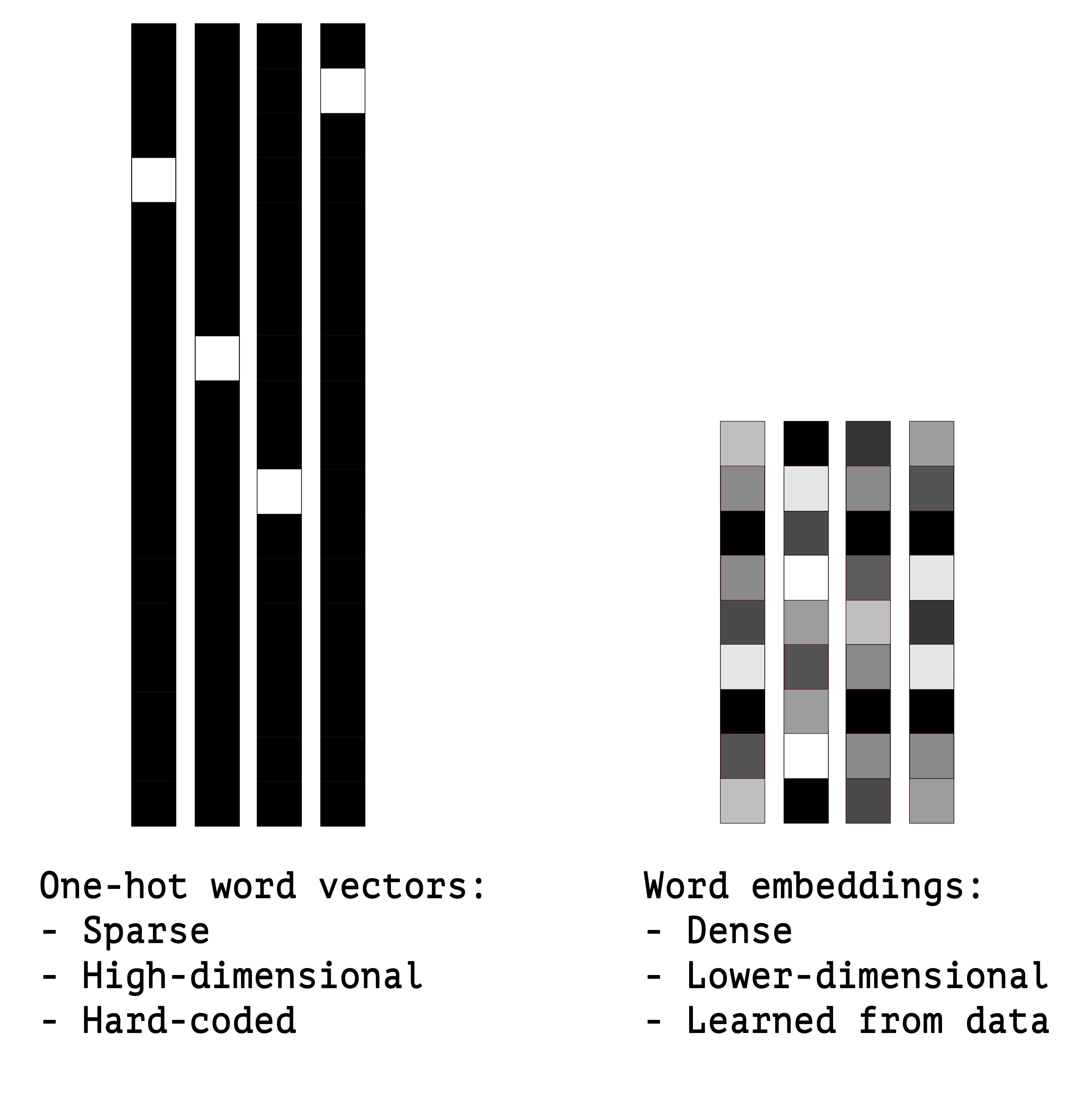
One-hot encoding vs Word embeddings, pc source
Continuous dense embedding can help to alleviate the curse of dimensionality. The biggest jump in NLP when moving from the sparse-input linear models to neural-network based models is to represent each feature as a dense vectors rather than one-hot encoding. One of the advantages of word embedding is the ability to generalize: semantically similar words are similar in vector, thus are closer to each other in the vector space. Additionally. It can reveal the hidden semantic relationship between words by their relative positions in the vector space. One notable example is that $v(“king”)-v(“man”)+v(“woman”)$ should be close to $v(“queen”)$.
In general, the word embeddings can be obtained through model training process, or alternatively we can use pre-trained models to get the embedding for free.
How to use word embedding?
Let’s imagine if we already have word embedding. How can we use it? Word embedding can be used as input feature for each word, usually concatenated or aggregated according to the model structure. Here is an example from the Primer of general structure for an NLP classification system based on a feed-forward neural network:
- Extract a set of core linguistic features $f_{1}, . . . , f_{k}$ that are relevant for predicting the output class.
- For each feature $f_{i}$ of interest, retrieve the corresponding vector $v(f_{i})$. (Here we can use the word embedding as the vector $v(f_{i})$ for each feature)
- Combine the vectors (either by concatenation, summation or a combination of both) into an input vector $x$.
- Feed $x$ into a non-linear classifier (feed-forward neural network).
How to learn word embedding?
To learn the word embedding, for most methods, it’s like training other parameters in the neural network. The word embeddings is the hidden layer that is optimized by predicting a target word given context words (CBOW), or predicting a word being a context word for the given target (Skip-gram model, used in Word2vec).
In general there are two main modeling approaches to learn the word enbeddings, count-based and context-based.
Count-Based model
Count-based methods utilize word frequency count and co-occurance matrix (similar to the co-occurance matrix in recommendation system). The idea is that words in the same contexts are more likely to be similar in semantic meanings.
-
CS224N hw1 on co-occurance here
Context-Based model
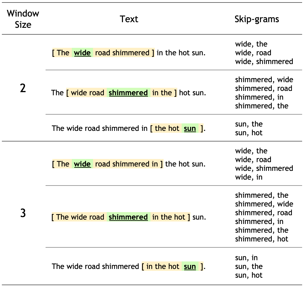
- Skip-Gram
- Continuous Bag-of-words
Context-based methods converted the problem into a predictive model (similar to predictive approach in recommendation system) that predict the central word given context words, or the other way around. While training the models, the word representation is learned as the model parameters. Some of the context-based models are Skip-Gram model, Continuous Bag-of-Words (CBOW) model.
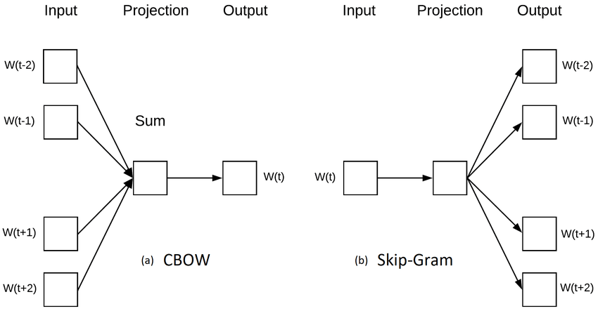
Continuous Bag-of-words (CBOW)
The Continuous Bag-of-words representation (Mikolov, Chen, Corrado, & Dean, 2013) is very similar to the traditional bag-of-words representation in which we discard order information, and works by either summing or averaging the embedding vectors of the corresponding features:
\[a\]Skip-Gram
TBA
Word2Vec
Word2Vec (Mikolov et al., 2013) is a popular technique to learn word embeddings using a two-layer neural net. It was introduced by a team of researchers at Google led by Tomas Mikolov. Google hosted a open source version of the Word2Vec model here.
- hw2 on implementing word2vec here
Loss Functions
TBA
Nagative Sampling
TBA
GloVe
Global Vector (GloVe) model tries to combine count-based Matrix Factorization and skip-gram model.
Related paper and note
Word2Vec, 2013
-
Distributed Representations of Words and Phrases and their Compositionality
-
Efficient Estimation of Word Representations in Vector Space
-
word2vec Parameter Learning Explained (This summary paper helped explain the detailed of CBOW and Skip-Gram models and herachical softmax and negative sampling)
The first two paper is about the primary Word2Vec model. The third paper served as a summary/note to further explain the word2vec model in the previous paper. Specifically on negative sampling (drawn by unigram distribution to the power of 3/4) based on skip-gram model, and its ojective function. Note that the words and contexts representation are learned jointly so the model is non-convex(comparing to learning only the word representation while fixing contexts, it will reduced to a logistic regression which is convex).
Here is a interesting Q&A quoted from the paper:
Why does this produce good word representations?
Good question. We don’t really know. The distributional hypothesis states that words in similar contexts have similar meanings. The objective above clearly tries to increase the quantity $v_{w} v_{c}$ for good word-context pairs, and decrease it for bad ones. Intuitively, this means that words that share many contexts will be similar to each other (note also that contexts sharing many words will also be similar to each other). This is, however, very hand-wavy. Can we make this intuition more precise? We’d really like to see something more formal.
Up Next: I will post some learning notes about NLP, especially about Transformer family and Attention Mechanism. Stay tuned!
Leave a comment